Extract Raster Values with Vector Data

Extracting raster values of pixels overlapping with vector data is one of the most common tasks for developers of earth observation applications. This notebook shows on the basis of a small toy dataset how to perform this task in Python with the eobox package.

In general there are tow two main approaches to solve this task in Python. (I am eager to know if you see another approach or additional advantages or disadvantages that should be added to this list.)

1. The rasterstats-way:

   • For each feature (point, line, polygon) in the vector dataset

     • get the geometry of the feature,

     • get the bounding box for that geometry,

     • get the raster data corresponding to the bounding box as array (extraction core),

     • rasterize the geometry such that it correponds to the array,

     • return only the raster values overlapping with the rasterized geometry.

A way of doing this in Python can be found in the gen_zonal_stats function implemented in the rasterstats package.

2. The rasterize-way:

   • Rasterize the whole vector dataset such that the rasterized raster matches the raster data from which to extract the values (e.g. with the gdal_rasterize function).

   • load the rasterized data as array and create a mask,

   • load the raster from which to extract the data as array and select the values to be kept by the mask.

This tutorial shows how to use the extract function implemented in the eobox package to go this way.

There is a major difference between the two approaches which might help you to find the best for your case: The first approach is memory sparing since the whole raster does not need to be loaded in memory at once, which is necessary in the second approach. However, if your vector dataset contains many features, it might be much faster to go for the second approach since it is not necessary to loop through all the features in Python.

Let’s get stated and import the required modules.

%load_ext autoreload
%autoreload 2
%matplotlib inline

import fnmatch
import geopandas as gpd
import os
import pandas as pd
from pathlib import Path

from eobox.raster import extraction
from eobox.raster.extraction import convert_df_to_geodf
from eobox import sampledata

We now load a small sample dataset from which we can derive all requird arguments for running the extract function.

Note that the sample dataset is S2 L1C that comes in different resolutions. Extraction from multiple resolutions is not supported and handling it is (so far) the responsibilit of the user.

Here we only slect the 10m bands for extraction.

dataset = sampledata.get_dataset("s2l1c")

src_vector = dataset["vector_file"]
burn_attribute = "pid"  # should be unique for the polygons and not contain zero
src_raster = fnmatch.filter(dataset["raster_files"], "*B0[2,3,4,8]*")  # 10 m bands
dst_names = ["_".join(Path(src).stem.split("_")[1::]) for src in src_raster]
extraction_dir = Path("s2l1c_ref__s2l1c/s2_l1c/10m")

print("***ARGUMENTS***")
print("\nsrc_vector:\n-----------\n -", src_vector)
print("\ndst_dir:\n--------\n -", extraction_dir)
print("\nsrc_raster:\n-----------\n -", "\n - ".join(src_raster))
print("\ndst_names:\n----------\n -", "\n - ".join(dst_names))
print("\n***ARGUMENTS - END***")

***ARGUMENTS***

src_vector:
-----------
 - /home/ben/Devel/Packages/eo-box/eobox/sampledata/data/s2l1c/s2l1c_ref.gpkg

dst_dir:
--------
 - s2l1c_ref__s2l1c/s2_l1c/10m

src_raster:
-----------
 - /home/ben/Devel/Packages/eo-box/eobox/sampledata/data/s2l1c/IMG_DATA/T33UUU_20170216T102101_B08.jp2
 - /home/ben/Devel/Packages/eo-box/eobox/sampledata/data/s2l1c/IMG_DATA/T33UUU_20170216T102101_B02.jp2
 - /home/ben/Devel/Packages/eo-box/eobox/sampledata/data/s2l1c/IMG_DATA/T33UUU_20170216T102101_B03.jp2
 - /home/ben/Devel/Packages/eo-box/eobox/sampledata/data/s2l1c/IMG_DATA/T33UUU_20170216T102101_B04.jp2

dst_names:
----------
 - 20170216T102101_B08
 - 20170216T102101_B02
 - 20170216T102101_B03
 - 20170216T102101_B04

***ARGUMENTS - END***

The vector dataset looks as follows:

gdf = gpd.read_file(src_vector)
gdf.plot(column="cid", figsize=(18, 8))

<matplotlib.axes._subplots.AxesSubplot at 0x7f20f4505c50>

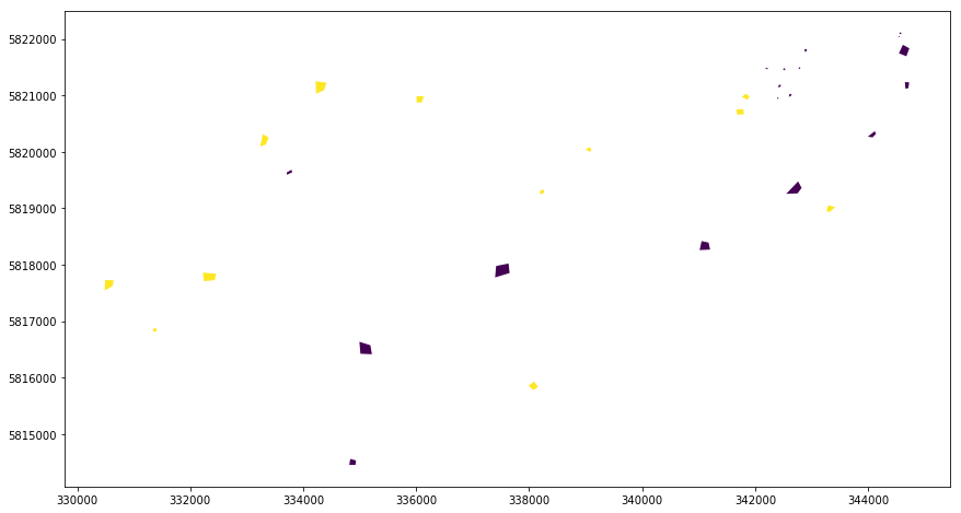
Note that the cid column represents the classes water (cid:1) and forest (cid:2). Even though we are usually interested in such an attribute we use as burn attribute the pid column contains unique ids for the polygons. Using a unique id for each feature is recommended since it assures that for each extracted pixel the polygon it belongs to can easily been identified. We will see later that it is easy to merge the cid information or any other information of the vector data attribute table can easily be merged into the extrected data.

But now let’s do the extraction.

%%time
extraction.extract(src_vector=src_vector,
                   burn_attribute=burn_attribute,
                   src_raster=src_raster,
                   dst_names=dst_names,
                   dst_dir=extraction_dir)

100%|██████████| 4/4 [00:00<00:00, 11.67it/s]

CPU times: user 2.18 s, sys: 343 ms, total: 2.53 s
Wall time: 397 ms

0

So what just happened? - Roughly the function made what was described above under the rasterize-way and stored the extracted data and some auxiliary information to .npy files:

list(extraction_dir.glob("*.npy"))

[PosixPath('s2l1c_ref__s2l1c/s2_l1c/10m/aux_coord_x.npy'),
 PosixPath('s2l1c_ref__s2l1c/s2_l1c/10m/20170216T102101_B04.npy'),
 PosixPath('s2l1c_ref__s2l1c/s2_l1c/10m/20170216T102101_B02.npy'),
 PosixPath('s2l1c_ref__s2l1c/s2_l1c/10m/aux_coord_y.npy'),
 PosixPath('s2l1c_ref__s2l1c/s2_l1c/10m/20170216T102101_B08.npy'),
 PosixPath('s2l1c_ref__s2l1c/s2_l1c/10m/aux_vector_pid.npy'),
 PosixPath('s2l1c_ref__s2l1c/s2_l1c/10m/20170216T102101_B03.npy')]

Note that the aux(iliary) variables are * aux_coord_x: the x coordinates of the pixels, * aux_coord_y: the y coordinates of the pixels, * aux_coord_y: the polygon id (here) or whatever attribute has been passed burn_attribute before.

The rest of the variables contain the data extracted from the raster layers.

• 20170216T102101_B02.npy

• 20170216T102101_B03.npy

• 20170216T102101_B04.npy

• 20170216T102101_B08.npy

It is worth noting that the function checks what has already been extracted by using the dst_names. Thus, only the dst_names that alread exist are skipped. So far, it is the responsibility of the user to delete existing bands in case they should be re-extracted.

With the the function load_extracted it is easy to load the data. It has a couple of options which returns different dataframes:

• The defaults return all variable in columns.

• patterns can be used to load specific variables matching a list of patterns.

extraction.load_extracted(extraction_dir, patterns=["aux_*.npy"]).head()

	aux_coord_x	aux_coord_y	aux_vector_pid
0	344545.0	5822035.0	17
1	344555.0	5822035.0	17
2	344615.0	5821885.0	6
3	344625.0	5821885.0	6
4	344615.0	5821875.0	6

extraction.load_extracted(extraction_dir, patterns=["aux_vector_pid.npy", "*_B??.npy"]).head()

	aux_vector_pid	20170216T102101_B04	20170216T102101_B02	20170216T102101_B08	20170216T102101_B03
0	17	928	1456	672	1072
1	17	928	1392	672	1040
2	6	928	1456	608	1072
3	6	864	1424	608	1072
4	6	928	1424	608	1072

• vars_in_cols can be used to load the variables in the columns.

  This does not make so much sense here, but if you have e.g. a long time series of the NDVI and you want to make time series analysis you might want to have the dates in the rows.

extraction.load_extracted(extraction_dir, patterns=["*B??.npy"], vars_in_cols=False).head()

	0	1	2	3	4	5	6	7	8	9	...	3490	3491	3492	3493	3494	3495	3496	3497	3498	3499
20170216T102101_B04	928	928	928	864	928	864	864	864	864	928	...	880	912	880	848	848	848	816	816	816	816
20170216T102101_B02	1456	1392	1456	1424	1424	1424	1424	1392	1424	1392	...	1448	1464	1448	1432	1448	1480	1432	1448	1400	1400
20170216T102101_B08	672	672	608	608	608	608	608	608	608	608	...	624	656	592	560	592	592	592	560	560	560
20170216T102101_B03	1072	1040	1072	1072	1072	1072	1040	1040	1040	1072	...	1056	1120	1056	1056	1056	1056	1056	1056	1056	1056

4 rows × 3500 columns

You can also get the head of the data loaded by load_extracted, i.e. the first five rows.

extraction.load_extracted(extraction_dir, vars_in_cols=False, head=True)

	0	1	2	3	4	5
aux_coord_x	344545.0	344555.0	344615.0	344625.0	344615.0	344625.0
20170216T102101_B04	928.0	928.0	928.0	864.0	928.0	864.0
20170216T102101_B02	1456.0	1392.0	1456.0	1424.0	1424.0	1424.0
aux_coord_y	5822035.0	5822035.0	5821885.0	5821885.0	5821875.0	5821875.0
20170216T102101_B08	672.0	672.0	608.0	608.0	608.0	608.0
aux_vector_pid	17.0	17.0	6.0	6.0	6.0	6.0
20170216T102101_B03	1072.0	1040.0	1072.0	1072.0	1072.0	1072.0

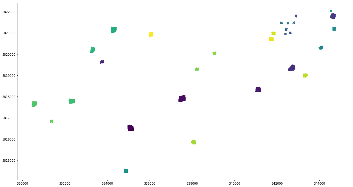
And finally you can convert the data to a geodataframe.

df_extracted = extraction.load_extracted(extraction_dir, patterns=["aux_*.npy", "*_B??.npy"])
gdf_extracted = convert_df_to_geodf(df_extracted, crs=extraction_dir)
gdf_extracted.plot(column='aux_vector_pid', marker='x', figsize=(20, 12))

<matplotlib.axes._subplots.AxesSubplot at 0x7f20bc8b81d0>

It has been said above that it is easy to join the extracted values to the values stored in the attribute table of the vector file.

df_extracted = df_extracted.merge(gdf[["pid", "cid", "comment"]], how="left", left_on="aux_vector_pid", right_on="pid")
df_extracted.head()

	aux_coord_x	aux_coord_y	aux_vector_pid	20170216T102101_B04	20170216T102101_B02	20170216T102101_B08	20170216T102101_B03	geometry	pid	cid	comment
0	344545.0	5822035.0	17	928	1456	672	1072	POINT (344545 5822035)	17	1	partially out; expecting: 2 - with default ras...
1	344555.0	5822035.0	17	928	1392	672	1040	POINT (344555 5822035)	17	1	partially out; expecting: 2 - with default ras...
2	344615.0	5821885.0	6	928	1456	608	1072	POINT (344615 5821885)	6	1	None
3	344625.0	5821885.0	6	864	1424	608	1072	POINT (344625 5821885)	6	1	None
4	344615.0	5821875.0	6	928	1424	608	1072	POINT (344615 5821875)	6	1	None

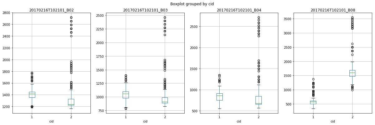
And now you can start analyzing the data.

import matplotlib.pyplot as plt
fig, axes = plt.subplots(1, 4, figsize=(20, 6))
for ax, var in zip(axes.flatten(), ["20170216T102101_B02", "20170216T102101_B03", "20170216T102101_B04", "20170216T102101_B08"]):
    df_extracted.boxplot(column=var, by="cid", ax=ax)